


All language is but a poor translation.
–Franz Kafka
Sometimes data lives in formats that take extra work to ingest. For common and explicitly data-oriented formats, common libraries already have readers built into them. Data frame libraries, for example, read a huge number of different file types. At worst, slightly less common formats have their own more specialized libraries that provide a relatively straightforward path between the original format and the general purpose data processing library you wish to use.
A greater difficulty often arises because a given format is not per se a data format, but exists for a different purpose. Nonetheless, often there is data somehow embedded or encoded in the format that we would like to utilize. For example, web pages are generally designed for human readers and rendered by web browsers with "quirks modes" that deal with not-quite-HTML, as is often needed. Portable Document Format (PDF) documents are similar in having intended human readers in mind, and yet also often containing tabular or other data that we would like to process as data scientists. Of course, in both cases, we would rather have the data itself in some separate, easily ingestible, format; but reality does not always live up to our hopes. Image formats likewise are intended for presentation of pictures to humans; but we sometimes wish to characterize or analyze collections of images in some data science or machine learning manner. There is a bit of a difference between Hypertext Markup Language (HTML) and PDF on one hand, and images on the other hand. With the former, we hope to find tables or numeric lists that are incidentally embedded inside a textual document. With the images, we are interested in the format itself as data: what is the pattern of pixel values and what does that tell us about characteristics of the image as such?
Still other formats are indeed intended as data formats, but they are unusual enough that common readers for the formats will not be available. Generally, custom text formats are manageable, especially if you have some documentation of what the rules of the format are. Custom binary formats are usually more work, but possible to decode if the need is sufficiently pressing and other encodings do not exist. Mostly such custom formats are legacy in some way, and a one-time conversion to more widely used formats is the best process.
Before we get to the sections of this chapter, let us run our standard setup code.
from src.setup import *
%load_ext rpy2.ipython
%%capture --no-stdout err
%%R
library(imager)
library(tidyverse)
library(rvest)
Important letters which contain no errors will develop errors in the mail.
–Anonymous
Concepts:
A great deal of interesting data lives on web pages, and often, unfortunately, we do not have access to the same data in more structured data formats. In the best cases, the data we are interested in at least lives within HTML tables inside of a web page; however, even where tables are defined, often the content of the cells has more than only the numeric or categorical values of interest to us. For example, a given cell might contain commentary on the data point or a footnote providing a source for the information. At other times, of course, the data we are interested in is not in HTML tables at all, but structured in some other manner across a web page.
In this section, we will first use the R library rvest to extract some tabular data, then use BeautifulSoup in Python to work with some non-tabular data. This shifting tool choice is not because one tool or the other is uniquely capable of doing the task we use it for, nor even is one necessarily better than the other at it. I simply want to provide a glimpse into a couple different tools for performing a similar task.
In the Python world, the framework Scrapy is also widely used—it does both more and less than BeautifulSoup. Scrapy can actually pull down web pages, and navigate dynamically amongst them while BeautifulSoup is only interested in the parsing aspect, and it assumes you have used some other tool or library (such as Requests) to actually obtain the HTML resource to be parsed. For what it does, BeautifulSoup is somewhat friendlier and is remarkably well able to handle malformed HTML. In the real world, what gets called "HTML" is often only loosely conformant to any actual format standards, and hence web browsers, for example, are quite sophisticated (and complicated) in providing reasonable rendering of only vaguely structured tag soups.
At the time of this writing, in 2020, the Covid-19 pandemic is ongoing, and the exact contours of the disease worldwide are changing on a daily basis. Given this active change, the current situation is too much of a moving target to make a good example (and too politically and ethically laden). Let us look at some data from a past disease though to illustrate web scraping. While there are surely other sources for similar data we could locate, and some are most likely in immediately readable formats, we will collect our data from the Wikipedia article on the 2009 flu pandemic.
A crucial fact about web pages is that they can be and often are modified by their maintainers. There are times when the Wayback Machine (https://archive.org/web/) can be used to find specific historical versions. Data that is available at a given point in time may not continue to be in the future at a given URL. Or even where a web page maintains the same underlying information, it may change details of its format that would change the functionality of our scripts for processing the page. On the other hand, many changes represent exactly the updates in data values that are of interest to us, and the dynamicness of a web page is exactly its greatest value. These are tradeoffs to keep in mind when scraping data from the web.
Wikipedia has a great many virtues, and one of them is its versioning of its pages. While a default URL for a given topic has a friendly and straightforward spelling that can often even be guessed from the name of a topic, Wikipedia also provides a URL parameter in its query strings that identifies an exact version of the web page that should remain bitwise identical for all time. There are a few exceptions to this permanence; for example, if an article is deleted altogether it may become inaccessible. Likewise if a template is part of a renaming, as unfortunately occured during the writing of this book, a "permanent" link can break. Let us examine the Wikipedia page we will attempt to scrape in this section.
# Same string composed over two lines for layout
# XXXX substituted for actual ID because of discussed breakage
url2009 = ("https://en.wikipedia.org/w/index.php?"
           "title=2009_flu_pandemic&oldid=XXXX")
The particular part of that previous page that we are interested in is an infobox about halfway down the article. It looks like this in my browser:
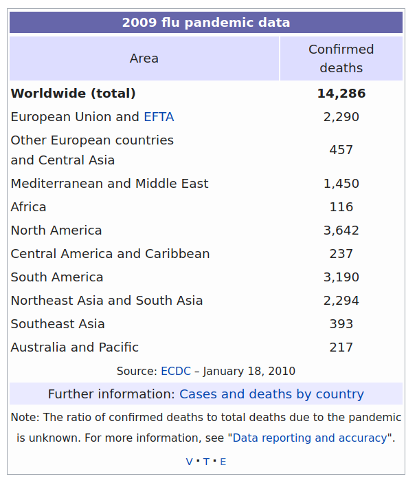
Image: Wikipedia Infobox in Article "2009 Flu Pandemic"
Constructing a script for web scraping inevitably involves a large amount of trial-and-error. In concept, it might be possible to manually read the underlying HTML before processing it, and correctly identify the positions and types of the element of interest. In practice, it is always quicker to eyeball the partially filtered or indexed elements, and refine the selection through repetition. For example, in this first pass, I determined that the "cases by region" table was number 4 on the web page by enumerating through earlier numbers and visually ruling them out. As rendered by a web browser, it is not always apparent what element is a table; it is also not necessarily the case that an elements being rendered visually above another actually occurs earlier in the underlying HTML.
This first pass also already performs a little bit of cleanup in value names. Through experimentation, I determined that some region names contain an HTML <br/> which is stripped in the below code, leaving no space between words. In order to address that, I replace the HTML break with a space, then need to reconstruct an HTML object from the string and select the table again.
page <- read_html(url2009)
table <- page %>%
    html_nodes("table") %>%
    .[[4]] %>%
    str_replace_all("<br>", " ") %>%
    minimal_html() %>%
    html_node("table") %>%
    html_table(fill = TRUE)
head(table, 3)
This code produced the following (before the template change issue):
   2009 flu pandemic data 2009 flu pandemic data 2009 flu pandemic data
1                    Area       Confirmed deaths                   <NA>
2       Worldwide (total)                 14,286                   <NA>
3 European Union and EFTA                  2,290                   <NA>
Although the first pass still has problems, all the data is basically present, and we can clean it up without
needing to query the source further. Because of the nested tables, the same header is incorrectly deduced
for
each column. The more accurate headers are relegated to the first row. Moreover, an extraneous column that
contains footnotes was created (it has content in some rows below those shown by head()).
Because
of the commas in numbers over a thousand, integers were not inferred. Let us convert the data.frame to a
tibble
data <- as_tibble(table,
        .name_repair = ~ c("Region", "Deaths", "drop")) %>%
    select(-drop) %>%
    slice(2:12) %>%
    mutate(Deaths = as.integer(gsub(",", "", Deaths)),
           Region = as.factor(Region))
data
And this might give us a helpful table like:
# A tibble: 11 x 2
   Region                                    Deaths
   <fct>                                      <int>
 1 Worldwide (total)                          14286
 2 European Union and EFTA                     2290
 3 Other European countries and Central Asia    457
 4 Mediterranean and Middle East               1450
 5 Africa                                       116
 6 North America                               3642
 7 Central America and Caribbean                237
 8 South America                               3190
 9 Northeast Asia and South Asia               2294
10 Southeast Asia                               393
11 Australia and Pacific                        217
Obviously this is a very small example that could easily be typed in manually. The general techniques shown might be applied to a much larger table. More significantly, they might also be used to scrape a table on a web page that is updated frequently. 2009 is strictly historical, but other data is updated every day, or even every minute, and a few lines like the ones shown could pull down current data each time it needs to be processed.
For our processing of a non-tabular source, we will use Wikipedia as well. Again, a topic that is of wide interest and not prone to deletion is chosen. Likewise, a specific historical version is indicated in the URL, just in case the page changes its structure by the time you read this. In a slightly self-referential way, we will look at the article that lists HTTP status codes in a term/definition layout. A portion of that page renders in my browser like this:
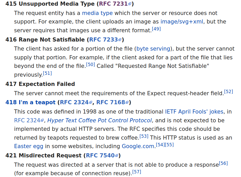
Image: HTTP Status Codes, Wikipedia Definition List
Numerous other codes are listed in the articles that are not in the screenshot. Moreover, there are section divisions and other descriptive elements or images throughout the page. Fortunately, Wikipedia tends to be very regular and predictable in its use of markup. The URL we will examine is:
url_http = ("https://en.wikipedia.org/w/index.php?"
            "title=List_of_HTTP_status_codes&oldid=947767948")
The first thing we need to do is actually retrieve the HTML content. The Python standard library module
urllib is perfectly able to do this task. However, even its official
documentation recommends using the third-party package Requests for most purposes. There is nothing
you
cannot do with urllib, but often the API is more difficult to use, and is
unnecessarily
complicated for historical/legacy reasons. For simple things, like what is shown in this book, it makes
little
difference; for more complicated tasks, getting in the habit of using Requests is a good idea. Let us open a
page and check the status code returned.
import requests
resp = requests.get(url_http)
resp.status_code
200
The raw HTML we retrieved is not especially easy to work with. Even apart from the fact it is compacted to remove extra whitespace, the general structure is a "tag soup" with various things nested in various places, and in which basic string methods or regular expressions do not help us very much in identifying the parts we are interested in. For example, here is a short segment from somewhere in the middle.
pprint(resp.content[43400:44000], width=55)
(b'e_ref-44" class="reference"><a href="#cite_note-' b'44">[43]</a></sup></dd>\n<dt><span class=' b'"anchor" id="412"></span>412 Precondition Failed' b' (<a class="external mw-magiclink-rfc" rel="nofo' b'llow" href="https://tools.ietf.org/html/rfc7232"' b'>RFC 7232</a>)</dt>\n<dd>The server does not meet' b' one of the preconditions that the requester put' b' on the request header fields.<sup id="cite_ref-' b'45" class="reference"><a href="#cite_note-45">&#' b'91;44]</a></sup><sup id="cite_ref-46" class=' b'"reference"><a href="#cite_note-46">[45]' b'</a></sup></dd>\n<dt><span class="anchor" id="413' b'"></span>413 Payload Too')
What we would like is to make the tag soup beautiful instead. The steps in doing so are first creating a "soup" object from the raw HTML, then using methods of that soup to pick out the elements we care about for our data set. As with the R and rvest version—as indeed, with any library you decide to use—finding the right data in the web page will involve trial-and-error.
from bs4 import BeautifulSoup
soup = BeautifulSoup(resp.content)
As a start at our examination, we noticed that the status codes themselves are each contained within an HTML <dt> element. Below we display the first and last few of the elements identified by this tag. Everything so identified is, in fact, a status code, but I only know that from manual inspection of all of them (fortunately, eyeballing fewer than 100 items is not difficult; doing so with a million would be infeasible). However, if we look back at the original web page itself, we will notice that two AWS custom codes at the end are not captured because the page formatting is inconsistent for those. In this section, we will ignore those, having determined they are not general purpose anyway.
codes = soup.find_all('dt')
for code in codes[:5] + codes[-5:]:
    print(code.text)
100 Continue
101 Switching Protocols
102 Processing (WebDAV; RFC 2518)
103 Early Hints (RFC 8297)
200 OK
524 A Timeout Occurred
525 SSL Handshake Failed
526 Invalid SSL Certificate
527 Railgun Error
530
It would be nice if each <dt> were matched with a corresponding <dd>. If it were, we could just read all the <dd> definitions and zip them together with the terms. Real-world HTML is messy. It turns out—and I discovered this while writing, not by planning the example—that there are sometimes more than one (and potentially sometimes zero) <dd> elements following each <dt>. Our goal then will be to collect all of the <dd> elements that follow a <dt> until other tags occur.
In the BeautifulSoup API, the empty space between elements is a node of plain text that contains exactly the
characters (including whitespace) inside that span. It is tempting to use the API
node.find_next_siblings() in this task. We could succeed doing this, but this method
will
fetch too much, including all subsequent <dt> elements after the current one. Instead, we can use the
property .next_sibling to get each one, and stop when needed.
def find_dds_after(node):
    dds = []
    sib = node.next_sibling
    while True:     # Loop until a break
        # Last sibling within page section
        if sib is None:
            break
        # Text nodes have no element name
        elif not sib.name:
            sib = sib.next_sibling
            continue
        # A definition node
        if sib.name == 'dd':
            dds.append(sib)
            sib = sib.next_sibling
        # Finished <dd> the definition nodes
        else:
            break
    return dds
The custom function I wrote above is straightforward, but special to this purpose. Perhaps it is extensible to similar definition lists one finds in other HTML documents. BeautifulSoup provides numerous useful APIs, but they are building blocks for constructing custom extractors rather than foreseeing every possible structure in an HTML document. To understand it, let us look at a couple of the status codes.
for code in codes[23:26]:
    print(code.text)
    for dd in find_dds_after(code):
        print("  ", dd.text[:40], "...")
400 Bad Request
   The server cannot or will not process th ...
401 Unauthorized (RFC 7235)
   Similar to 403 Forbidden, but specifical ...
   Note: Some sites incorrectly issue HTTP  ...
402 Payment Required
   Reserved for future use. The original in ...
The HTTP 401 response contains two separate definition blocks. Let us apply the function across all the HTTP code numbers. What is returned is a list of definition blocks; for our purpose we will join the text of each of these with a newline. In fact, we construct a data frame with all the information of interest to us in the next cells.
data = []
for code in codes:
    # All codes are 3 character numbers
    number = code.text[:3]
    # parenthetical is not part of status
    text, note = code.text[4:], ""
    if " (" in text:
        text, note = text.split(" (")
        note = note.rstrip(")")
    # Compose description from list of strings
    description = "\n".join(t.text for t in find_dds_after(code))
    data.append([int(number), text, note, description])
From the Python list of lists, we can create a Pandas DataFrame for further work on the data set.
(pd.DataFrame(data,
              columns=["Code", "Text", "Note", "Description"])
    .set_index('Code')
    .sort_index()
    .head(8))
| Text | Note | Description | |
|---|---|---|---|
| Code | |||
| 100 | Continue | The server has received the request headers an... | |
| 101 | Switching Protocols | The requester has asked the server to switch p... | |
| 102 | Processing | WebDAV; RFC 2518 | A WebDAV request may contain many sub-requests... |
| 103 | Checkpoint | Used in the resumable requests proposal to res... | |
| 103 | Early Hints | RFC 8297 | Used to return some response headers before fi... |
| 200 | OK | Standard response for successful HTTP requests... | |
| 201 | Created | The request has been fulfilled, resulting in t... | |
| 202 | Accepted | The request has been accepted for processing, ... |
Clearly, the two examples this book walked through in some details are not general to all the web pages you
may
wish to scrape data from. Organization into tables and into definition lists are certainly two common uses
of
HTML to represent data, but many other conventions might be used. Particular domain specific—or likely page
specific—class and id attributes on elements is also a common way to mark the
structural role of different data elements. Libraries like rvest, BeautifulSoup, and scrapy all make
identification and extraction of HTML by element attributes straightforward as well. Simply be prepared to
try
many variations on your web scraping code before you get it right. Generally, your iteration will be a
narrowing
process; each stage needs toinclude the information desired, it becomes a process of removing the
parts
you do not want through refinement.
Another approach that I have often used for web scraping is to use the command-line web browsers
lynx and links. Install either or both with your system package manager. These
tools
can dump HTML contents as text which is, in turn, relatively easy to parse if the format is simple. There
are
many times when just looking for patterns of intentation, vertical space, searching for particular keywords,
or
similar text processing, will get the data you need more quickly than the trial-and-error of parsing
libraries
like rvest or BeautifulSoup. Of course, there is always a certain amount of eyeballing and retrying
commands.
For people who are well versed in text processing tools, this approach is worth considering.
The two similar text-mode web browsers both share a -dump switch that outputs non-interactive
text
to STDOUT. Both of them have a variety of other switches that can tweak the rendering of the text in a
variety
of ways. The output from these two tools is similar, but the rest of your scripting will need to pay
attention
to the minor differences. Each of these browsers will do a very good job of dumping 90% of web pages as text
that is easy to process. Of the problem 10% (a hand waving percentage, not a real measure), often one or the
other tool will produce something reasonable to parse. In certain cases, one of these browsers may produce
useful results and the other will not. Fortunately, it is easy simply to try both for a given task or site.
Let us look at the output from each tool against a portion of the HTTP response code page. Obviously, I
experimented to find the exact line ranges of output that would correspond. You can see that only incidental
formatting differences exist in this friendly HTML page. First with lynx:
%%bash
base='https://en.wikipedia.org/w/index.php?title='
url="$base"'List_of_HTTP_status_codes&oldid=947767948'
lynx -dump $url | sed -n '397,406p'
          requester put on the request header fields.^[170][44]^[171][45]

413 Payload Too Large ([172]RFC 7231)
          The request is larger than the server is willing or able to
          process. Previously called "Request Entity Too Large".^[173][46]

414 URI Too Long ([174]RFC 7231)
          The [175]URI provided was too long for the server to process.
          Often the result of too much data being encoded as a
          query-string of a GET request, in which case it should be
And the same part of the page again, but this time with links:
%%bash
base='https://en.wikipedia.org/w/index.php?title='
url="$base"'List_of_HTTP_status_codes&oldid=947767948'
links -dump $url | sed -n '377,385p'
           requester put on the request header fields.^[44]^[45]

413 Payload Too Large (RFC 7231)
           The request is larger than the server is willing or able to
           process. Previously called "Request Entity Too Large".^[46]

414 URI Too Long (RFC 7231)
           The URI provided was too long for the server to process. Often the
           result of too much data being encoded as a query-string of a GET
The only differences here are one space difference in indentation of the definition element and some difference in the formatting of footnote links in the text. In either case, it would be easy enough to define some rules for the patterns of terms and their definitions. Something like this:
Let us wave goodbye to the Scylla of HTML, as we pass by, and fall into the Charybdis of PDF.
This functionary grasped it in a perfect agony of joy, opened it with a trembling hand, cast a rapid glance at its contents, and then, scrambling and struggling to the door, rushed at length unceremoniously from the room and from the house.
–Edgar Allan Poe
Concepts:
There are a great many commercial tools to extract data which has become hidden away in PDF (portable document format) files. Unfortunately, many organizations—government, corporate, and others—issue reports in PDF format but do not provide data formats more easily accessible to computer analysis and abstraction. This is common enough to have provided impetus for a cottage industry of tools for semi-automatically extracting data back out of these reports. This book does not recommend use of proprietary tools about which there is no guarantee of maintenance and improvement over time; as well, of course, those tools cost money and are an impediment to cooperation among data scientists who work together on projects without necessarily residing in the same "licensing zone."
There are two main elements that are likely to interest us in a PDF file. An obvious one is tables of data, and those are often embedded in PDFs. Otherwise, a PDF can often simply be treated as a custom text format, as we discuss in a section below. Various kinds of lists, bullets, captions, or simply paragraph text, might have data of interest to us.
There are two open source tools I recommend for extraction of data from PDFs. One of these it the
command-line
tool pdftotext which is part of the Xpdf and derived Poppler
software suites. The second is a Java tool called tabula-java. Tabula-java is in turn the
underlying engine for the GUI tool Tabula, and also has language bindings for Ruby
(tabula-extractor), Python (tabula-py), R (tabulizer),
and
Node.js (tabula-js). Tabula creates a small web server that allows interaction within a
browser
to do operations like creating lists of PDFs and selecting regions where tables are located. The Python and
R
bindings also allow direct creation of data frames or arrays, with the R binding incorporating an optional
graphical widget for region selection.
For this discussion, we do not use any of the language bindings, nor the GUI tools. For one-off selection of one-page data sets, the selection tools could be useful, but for automation of recurring document updates or families of similar documents, scripting is needed. Moreover, while the various language bindings are perfectly suitable for scripting, we can be somewhat more language agnostic in this section by limiting ourselves to the command-line tool of the base library.
As an example for this section, let us use a PDF that was output from the preface of this book itself. There may have been small wording changes by the time you read this, and the exact formatting of the printed book or ebook will surely be somewhat different from this draft version. However, this nicely illustrates tables rendered in several different styles that we can try to extract as data. There are three tables, in particular, which we would like to capture.
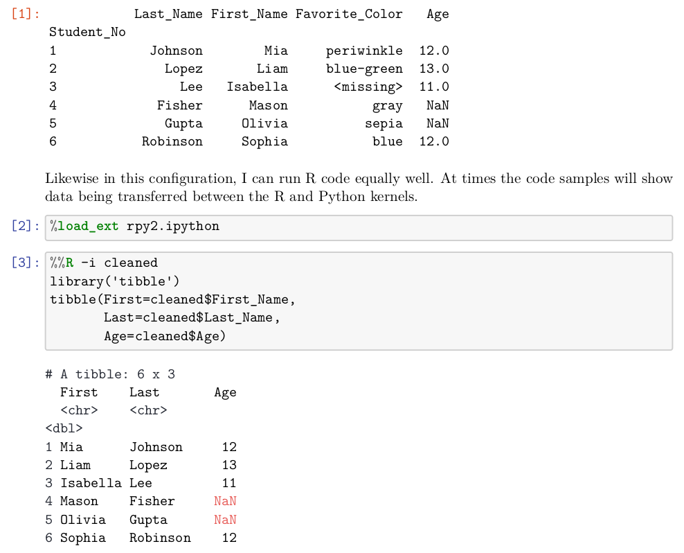
Image: Page 5 of Book Preface
On page 5 of the draft preface, a table is rendered by both Pandas and tibble, with corresponding minor presentation differences. On page 7 another table is included that looks somewhat different again.
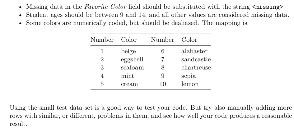
Image: Page 7 of Book Preface
Running tabula-java requires a rather long command line, so I have created a small bash script to wrap it on my personal system:
#!/bin/bash
# script: tabula
# Adjust for your personal system path
TPATH='/home/dmertz/git/tabula-java/target'
JAR='tabula-1.0.4-SNAPSHOT-jar-with-dependencies.jar'
java -jar "$TPATH/$JAR" $@
Extraction will sometimes automatically recognize tables per page with the --guess option, but
you
can get better control by specifying a portion of a page where tabula-java should look for a table. We
simply
output to STDOUT in the following code cells, but outputting to a file is just another option switch.
%%bash
tabula -g -t -p5 data/Preface-snapshot.pdf
[1]:,,Last_Name,First_Name,Favorite_Color,Age
"",Student_No,,,,
"",1,Johnson,Mia,periwinkle,12.0
"",2,Lopez,Liam,blue-green,13.0
"",3,Lee,Isabella,<missing>,11.0
"",4,Fisher,Mason,gray,NaN
"",5,Gupta,Olivia,sepia,NaN
"",6,Robinson,Sophia,blue,12.0
Tabula does a good, but not perfect, job. The Pandas style of setting the name of the index column below the other headers threw it off slightly. There is also a spurious first column that is usually empty strings, but has a header as the output cell number. However, these small defects are very easy to clean up, and we have a very nice CSV of the actual data in the table.
Remember from just above, however, that page 5 actually had two tables on it. Tabula-java only captured the first one, which is not unreasonable, but is not all the data we might want. Slightly more custom instructions (determined by moderate trial-and-error to determine the region of interest) can capture the second one.
%%bash
tabula -a'%72,13,90,100' -fTSV -p5 data/Preface-snapshot.pdf
First	Last	Age
<chr>	<chr>
bl>
Mia	Johnson	12
Liam	Lopez	13
Isabella	Lee	11
Mason	Fisher	NaN
Olivia	Gupta	NaN
Sophia	Robinson	12
To illustrate the output options, we chose tab-delimited rather than comma-separated for the output. A JSON output is also available. Moreover, by adjusting the left margin (as percent, but as typographic points is also an option), we can eliminate the unecessary row numbers. As before, the ingestion is good but not perfect. The tibble formatting of data type markers is superfluous for us. Discarding the two rows with unnecessary data is straightforward.
Finally for this example, let us capture the table on page 7 that does not have any of those data frame library extra markers. This one is probably more typical of the tables you will encounter in real work. For the example, we use points rather than page percentage to indicate the position of the table.
%%bash
tabula -p7 -a'120,0,220,500' data/Preface-snapshot.pdf
Number,Color,Number,Color
1,beige,6,alabaster
2,eggshell,7,sandcastle
3,seafoam,8,chartreuse
4,mint,9,sepia
5,cream,10,lemon
The extraction here is perfect, although the table itself is less than ideal in that it it repeats the number/color pairs twice. However, that is likewise easy enough to modify using data frame libraries.
The tool tabula-java, as the name suggests, is only really useful for identifying tables. In contrast, pdftotext creates a best-effort purely text version of a PDF. Most of the time this is quite good. From that, standard text processing and extraction techniques usually work well, including those that parse tables. However, since an entire document (or a part of it selected by pages) is output, that lets us work with other elements like bullet lists, raw prose, or other identifiable data elements of a document.
%%bash
# Start with page 7, tool writes to .txt file
# Use layout mode to preserve horizontal position
pdftotext -f 7 -layout data/Preface-snapshot.pdf
# Remove 25 spaces from start of lines
# Wrap other lines that are too wide
sed -E 's/^ {,25}//' data/Preface-snapshot.txt |
    fmt -s |
    head -20
• Missing data in the Favorite Color field should be substituted with
the string <missing>.
• Student ages should be between 9 and 14, and all other values are
considered missing data.
• Some colors are numerically coded, but should be dealiased. The
mapping is:

Number     Color      Number    Color
      1       beige          6     alabaster
      2       eggshell       7     sandcastle
      3       seafoam        8     chartreuse
      4       mint           9     sepia
      5       cream          10    lemon

Using the small test data set is a good way to test your code. But try
also manually adding more
rows with similar, or different, problems in them, and see how well your
code produces a reasonable
result.
The tabular part in the middle would be simple to read as a fixed width format. The bullets at top or the paragraph at bottom might be useful for other data extraction purposes. In any case, it is plain text at this point, which is easy to work with.
Let us turn now to analyzing images, mostly for their metadata and overall statistical characteristics.
As the Chinese say, 1001 words is worth more than a picture.
–John McCarthypicture
Concepts:
For certain purposes, raster images are themselves the data sets of interest to us. "Raster" just means rectangular collections of pixel values. The field of machine learning around image recognition and image processing is far outside the scope of this book. The few techniques in this section might be useful to get your data ready to the point of developing input to those tools, but no further than that. Also not considered in this book are other kinds of recognition of the content of images at a high-level. For example, optical character recognition (OCR) tools might recognize an image as containing various strings and numbers as rendered fonts, and those values might be the data we care about.
If you have the misfortune of having data that is only available in printed and scanned form, you most certainly have my deep sympathy. Scanning the images using OCR is likely to produce noisy results with many misrecognitions. Detecting those is addressed in chapter 4 (Anomaly Detection); essentially you will get either wrong strings or wrong numbers when these errors happen, ideally the errors will be identifiable. However, the specifics of those technologies are not within the current scope.
For this section, we merely want to present tools to read in images as numeric arrays, and perform a few basic processing steps that might be used in your downstream data analysis or modeling. Within Python, the libary Pillow is the go-to tool (backward compatible successor to PIL, which is deprecated). Within R, the imager library seems to be most widely used for the general purpose tasks of this section. As a first task, let us examine and describe the raster images used in the creation of this book.
from PIL import Image, ImageOps

for fname in glob('img/*'):
    try:
        with Image.open(fname) as im:
            print(fname, im.format, "%dx%d" % im.size, im.mode)
    except IOError:
        pass
img/(Ch03)Luminance values in Confucius drawing.png PNG 2000x2000 P
img/Flu2009-infobox.png PNG 607x702 RGBA
img/Konfuzius-1770.jpg JPEG 566x800 RGB
img/UMAP.png PNG 2400x2400 RGBA
img/(Ch02)108 ratings.png PNG 3600x2400 RGBA
img/DQM-with-Lenin-Minsk.jpg MPO 3240x4320 RGB
img/(Ch02)Counties of the United States.png PNG 4800x3000 RGBA
img/PCA Components.png PNG 3600x2400 RGBA
img/(Ch01)Student score by year.png PNG 3600x2400 RGBA
img/HDFCompass.png PNG 958x845 RGBA
img/(Ch01)Visitors per station (max 32767).png PNG 3600x2400 RGBA
img/t-SNE.png PNG 4800x4800 RGBA
img/dog_cat.png PNG 6000x6000 RGBA
img/Parameter space for two features.png PNG 3600x2400 RGBA
img/Whitened Components.png PNG 3600x2400 RGBA
img/(Ch01)Lengths of Station Names.png PNG 3600x2400 RGBA
img/preface-2.png PNG 945x427 RGBA
img/DQM-with-Lenin-Minsk.jpg_original MPO 3240x4320 RGB
img/PCA.png PNG 4800x4800 RGBA
img/Excel-Pitfalls.png PNG 551x357 RGBA
img/gnosis-traffic.png PNG 1064x1033 RGBA
img/Film_Awards.png PNG 1587x575 RGBA
img/HTTP-status-codes.png PNG 934x686 RGBA
img/preface-1.png PNG 988x798 RGBA
img/GraphDatabase_PropertyGraph.png PNG 2000x1935 RGBA
We see that mostly PNG images were used, with a smaller number of JPEGs. Each has certain spatial dimensions, by width then height, and each is either RGB, or RGBA if it includes an alpha channel. Other images might be HSV format. Converting between color spaces is easy enough using tools like Pillow and imager, but it is important to be aware of which model a given image uses. Let us read one in, this time using R.
%%R
library(imager)
confucius <- load.image("img/Konfuzius-1770.jpg")
print(confucius)
plot(confucius)
Image. Width: 566 pix Height: 800 pix Depth: 1 Colour channels: 3

Let us analyze the contours of the pixels.
We can work on getting a feel for the data, which at heart is simply an array of values, with some tools the library provides. In the case of imager which is built on CImg, the internal representation is 4-dimensional. Each plane is an X by Y grid of pixels (left-to-right, top-to-bottom). However, the format can represent a stack of images—for example, an animation—in the depth dimension. The several color channels (if the image is not grayscale) are the final dimension of the array. The Confucius example is a single image, so the third dimension is of length one. Let us look at some summary data about the image.
%%R
grayscale(confucius) %>%
    hist(main="Luminance values in Confucius drawing")

%%R
# Save histogram to disk
png("img/(Ch03)Luminance values in Confucius drawing.png", width=1200)
grayscale(confucius) %>%
    hist(main="Luminance values in Confucius drawing")
Perhaps we would like to look at the distribution only of one color channel instead.
%%R
B(confucius) %>%
    hist(main="Blue values in Confucius drawing")

%%R
# Save histogram to disk
png("img/(Ch03)Blue values in Confucius drawing.png", width=1200)
B(confucius) %>%
    hist(main="Blue values in Confucius drawing")
The histograms above simply utilize the standard R histogram function. There is nothing special about the fact that the data represents an image. We could perform whatever statistical tests or summarizations we wanted on the data to make sure it makes sense for our purpose; a histogram is only a simple example to show the concept. We can also easily transform the data into a tidy data frame. As of this writing, there is an "impedance error" in converting directly to a tibble, so the below cell uses an intermediate data.frame format. Tibbles are often but not always drop in replacements when functions were written to work with data.frame objects.
%%R
data <- as.data.frame(confucius) %>%
    as_tibble %>%
    # channels 1, 2, 3 (RGB) as factor
    mutate(cc = as.factor(cc))
data
# A tibble: 1,358,400 x 4
       x     y cc    value
   <int> <int> <fct> <dbl>
 1     1     1 1     0.518
 2     2     1 1     0.529
 3     3     1 1     0.518
 4     4     1 1     0.510
 5     5     1 1     0.533
 6     6     1 1     0.541
 7     7     1 1     0.533
 8     8     1 1     0.533
 9     9     1 1     0.510
10    10     1 1     0.471
# … with 1,358,390 more rows
With Python and PIL/Pillow, working with image data is very similar. As in R, the image is an array of pixel values with some metadata attached to it. Just for fun, we use a variable name with Chinese characters to illustrate that such is supported in Python.
# Courtesy name: Zhòngní (仲尼)
# "Kǒng Fūzǐ" (孔夫子) was coined by 16th century Jesuits
仲尼 = Image.open('img/Konfuzius-1770.jpg')
data = np.array(仲尼)
print("Image shape:", data.shape)
print("Some values\n", data[:2, :, :])
Image shape: (800, 566, 3)
Some values
 [[[132  91  69]
  [135  94  74]
  [132  91  71]
  ...
  [148  98  73]
  [142  95  69]
  [135  89  63]]

[[131  90  68]
  [138  97  75]
  [139  98  78]
  ...
  [147 100  74]
  [144  97  71]
  [138  92  66]]]
In the Pillow format, images are stored as 8-bit unsigned integers rather than as floating-point numbers in [0.0, 1.0] range. Converting between these is easy enough, of course, as is other normalization. For example, for many neural network tasks, the prefered representation is values centered at zero with standard deviation of one. The array used to hold Pillow images in 3-dimensional since it does not have provision for stacking multiple images in the same object.
It might be useful to perform manipulation of image data before processing. The below example is contrived, and similar to one used in the library tutorial. The idea in the next few code lines is that we will mask the image based on the values in the blue channel, but then use that to selectively zero-out red values. The result is not visually attractive for a painting, but one can imagine it might be useful for e.g. medical imaging or false-color radio astronomy images (I am also working around making a transformation that is easily visible in a monochrome book as well as in full color).
The convention used in the .paste() method is a bit odd. The rule is: Where the mask is 255,
copied
as is; where mask is 0, preserve current value (blend if intermediate). The effect overall in the color
version
is that in the mostly red-tinged image, the greens dominate at the edges where the image had been most red.
In
grayscale it mostly just darkens the edges.
# split the Confucius image into individual bands
source = 仲尼.split()
R, G, B = 0, 1, 2

# select regions where blue is less than 100
mask = source[B].point(lambda i: 255 if i < 100 else 0)
source[R].paste(0, None, mask)
im = Image.merge(仲尼.mode, source)
im.save('img/(Ch03)Konfuzius-bluefilter.jpg')
ImageOps.scale(im, 0.5)

The original in comparison.
ImageOps.scale(仲尼, 0.5)

Another example we mentioned is that transformation of the color space might be useful. For example, rather than look at colors red, green, and blue, it might be that hue, saturation, and lightness are better features for your modeling needs. This is a deterministic transformation of the data, but emphasizing different aspects. It is something analogous to the decompositions like principal component analysis that is discussed in chapter 7 (Feature Engineering). Here we convert from an RGB to HSL representation of the image.
%%R
confucius.hsv <- RGBtoHSL(confucius)
data <- as.data.frame(confucius.hsv) %>%
    as_tibble %>%
    # channels 1, 2, 3 (HSV) as factor
    mutate(cc = as.factor(cc))
data
# A tibble: 1,358,400 x 4
       x     y cc    value
   <int> <int> <fct> <dbl>
 1     1     1 1      21.0
 2     2     1 1      19.7
 3     3     1 1      19.7
 4     4     1 1      19.7
 5     5     1 1      19.7
 6     6     1 1      19.7
 7     7     1 1      19.7
 8     8     1 1      19.7
 9     9     1 1      19.7
10    10     1 1      20
# … with 1,358,390 more rows
Both the individual values and the shape of the space have changed in this transformation. The transformation is lossless, beyond minor rounding issues. A summary by channel will illustrate this.
%%R
data %>%
    mutate(cc = recode(
        cc, `1`="Hue", `2`="Saturation", `3`="Value")) %>%
    group_by(cc) %>%
    summarize(Mean = mean(value), SD = sd(value))
`summarise()` ungrouping output (override with `.groups` argument)
# A tibble: 3 x 3
  cc           Mean     SD
  <fct>       <dbl>  <dbl>
1 Hue        34.5   59.1
2 Saturation  0.448  0.219
3 Value       0.521  0.192
Let us look at perhaps the most important aspect of images to data scientists.
Photographic images may contain metadata embedded inside them. Specifically, the Exchangeable Image File Format (Exif) specifies how such metadata can be embedded in JPEG, TIFF, and WAV formats (the last is an audio format). Digital cameras typically add this information to the images they create, often including details such as timestamp and latitude/longitude location.
Some of the data fields within an Exif mapping are textual, numeric, or tuples; others are binary data. Moreover, the keys in the mapping are from ID numbers that are not meaningful to humans directly; this mapping is a published standard, but some equipment makers may introduce their own IDs as well. The binary fields contain a variety of types of data, encoded in various ways. For example, some cameras may attach small preview images as Exif metadata; but simpler fields are also encoded.
The below function will utilize Pillow to return two dictionaries, one for the textual data, the other for
the
binary data. Tag IDs are expanded to human readable names, where available. Pillow uses "camel case" for
these
names, but other tools have different variations on capitalization and punctuation within the tag names. The
casing by Pillow is what I like to call Bactrian case—as opposed to Dromedary case—both of which differ from
Python's usual "snake case" (e.g. BactrianCase versus dromedaryCase versus
snake_case).
from PIL.ExifTags import TAGS

def get_exif(img):
    txtdata, bindata = dict(), dict()
    for tag_id in (exifdata := img.getexif()):
        # Lookup tag name from tag_id if available
        tag = TAGS.get(tag_id, tag_id)
        data = exifdata.get(tag_id)
        if isinstance(data, bytes):
            bindata[tag] = data
        else:
            txtdata[tag] = data
    return txtdata, bindata
Let us check whether the Confucius image has any metadata attached.
get_exif(仲尼) # Zhòngní, i.e. Confucius
({}, {})
We see that this image does not have any such metadata. Let us look instead at a photograph taken of the author next to a Lenin statue in Minsk.
# Could continue using multi-lingual variable names by
# choosing `Ленин`, `Ульянов` or `Мінск`
dqm = Image.open('img/DQM-with-Lenin-Minsk.jpg')
ImageOps.scale(dqm, 0.1)

This image, taken with a digital camera, indeed has Exif metadata. These generally concern photographic settings, which are perhaps valuable to analyze in comparing images. This example also has a timestamp, although not in this case a latitude/longitude position (the camera used did not have a GPS sensor). Location data, where available, can obviously be valuable for many purposes.
txtdata, bindata = get_exif(dqm)
txtdata
{'CompressedBitsPerPixel': 4.0,
 'DateTimeOriginal': '2015:02:01 13:01:53',
 'DateTimeDigitized': '2015:02:01 13:01:53',
 'ExposureBiasValue': 0.0,
 'MaxApertureValue': 4.2734375,
 'MeteringMode': 5,
 'LightSource': 0,
 'Flash': 16,
 'FocalLength': 10.0,
 'ColorSpace': 1,
 'ExifImageWidth': 3240,
 'ExifInteroperabilityOffset': 10564,
 'FocalLengthIn35mmFilm': 56,
 'SceneCaptureType': 0,
 'ExifImageHeight': 4320,
 'Contrast': 0,
 'Saturation': 0,
 'Sharpness': 0,
 'Make': 'Panasonic',
 'Model': 'DMC-FH4',
 'Orientation': 1,
 'SensingMethod': 2,
 'YCbCrPositioning': 2,
 'ExposureTime': 0.00625,
 'XResolution': 180.0,
 'YResolution': 180.0,
 'FNumber': 4.4,
 'ExposureProgram': 2,
 'CustomRendered': 0,
 'ISOSpeedRatings': 500,
 'ResolutionUnit': 2,
 'ExposureMode': 0,
 34864: 1,
 'WhiteBalance': 0,
 'Software': 'Ver.1.0  ',
 'DateTime': '2015:02:01 13:01:53',
 'DigitalZoomRatio': 0.0,
 'GainControl': 2,
 'ExifOffset': 634}
One detail we notice in the textual data is that the tag ID 34864 was not unaliased by Pillow. I can locate
external documentation indicating that the ID should indicate "Exif.Photo.SensitivityType" but Pillow is
apparently unaware of that ID. The bytes strings may contain data you wish to utilize, but the meaning given
to
each field is different and must be compared to reference definitions. For example, the field
ExifVersion is defined as ASCII bytes, but not as UTF-8 encoded bytes like regular
text
field values. We can view that using:
bindata['ExifVersion'].decode('ascii')
'0230'
In contrast, the tag named ComponentsConfiguration consists of four bytes, with each byte
representing a color code. The function get_exif() produces separate text and binary
dictionaries
(txtdata and bindata). Let us decode bindata with a new special
function.
def components(cc):
    colors = {0: None,
              1: 'Y', 2: 'Cb', 3: 'Cr',
              4: 'R', 5: 'G', 6: 'B'}
    return [colors.get(c, 'reserved') for c in cc]
components(bindata['ComponentsConfiguration'])
['Y', 'Cb', 'Cr', None]
Other binary fields are encoded in other ways. The specifications are maintained by the Japan Electronic Industries Development Association (JEIDA). This section intends only to give you a feel for working with this kind of metadata, and is by no means a complete reference.
Let us turn our attention now to the specialize binary data formats we sometimes need to work with.
I usually solve problems by letting them devour me.
–Franz Kafka
Concepts:
There are a great many binary formats that data might live in. Everything very popular has grown good open source libraries, but you may encounter some legacy or in-house format for which this is not true. Good general advice is that unless there is an ongoing and/or performance sensitive need for processing an unusual format, try to leverage existing parsers. Custom formats can be tricky, and if one is uncommon, it is as likely as not also to be underdocumented.
If an existing tool is only available in a language you do not wish to use for your main data science work, nonetheless see if that can be easily leveraged to act only as as a means to export to a more easily accessed format. A fire-and-forget tool might be all you need, even if it is one that runs recurringly, but asynchronously with the actual data processing you need to perform.
For this section, let as assume that the optimistic situation is not realized, and we have nothing beyond some bytes on disk, and some possibly flawed documentation to work with. Writing the custom code is much more the job of a systems engineer than a data scientist; but we data scientists need to be polymaths, and we should not be daunted by writing a little bit of systems code.
For this relatively short section, we look at a simple and straightforward binary format. Moreover, this is a real-world data format for which we do not actually need a custom parser. Having an actual well-tested, performant, and bullet-proof parser to compare our toy code with is a good way to make sure we do the right thing. Specifically, we will read data stored in the NumPy NPY format, which is documented as follows (abridged):
\x93NUMPY.\x01.
\x00.
First, we read in some binary data using the standard reader, using Python and NumPy, to understand what type of object we are trying to reconstruct. It turns out that the serialization was of a 3-dimensional array of 64-bit floating-point values. A small size was chosen for this section, but of course real-world data will generally be much larger.
arr = np.load(open('data/binary-3d.npy', 'rb'))
print(arr, '\n', arr.shape, arr.dtype)
[[[ 0.  1.  2.]
  [ 3.  4.  5.]]

[[ 6.  7.  8.]
  [ 9. 10. 11.]]]
 (2, 2, 3) float64
Visually examining the bytes is a good way to have a better feel for what is going on with the data. NumPy is, of course, a clearly and correctly documented project; but for some hypothetical format, this is an opportunity to potentially identify problems with the documentation not matching the actual bytes. More subtle issues may arise in the more detailed parsing; for example, the meaning of bytes in a particular location can be contingent on flags occurring elsewhere. Data science is, in surprisingly large part, a matter of eyeballing data.
%%bash
hexdump -Cv data/binary-3d.npy
00000000  93 4e 55 4d 50 59 01 00  76 00 7b 27 64 65 73 63  |.NUMPY..v.{'desc|
00000010  72 27 3a 20 27 3c 66 38  27 2c 20 27 66 6f 72 74  |r': '<f8', 'fort|
00000020  72 61 6e 5f 6f 72 64 65  72 27 3a 20 46 61 6c 73  |ran_order': Fals|
00000030  65 2c 20 27 73 68 61 70  65 27 3a 20 28 32 2c 20  |e, 'shape': (2, |
00000040  32 2c 20 33 29 2c 20 7d  20 20 20 20 20 20 20 20  |2, 3), }        |
00000050  20 20 20 20 20 20 20 20  20 20 20 20 20 20 20 20  |                |
00000060  20 20 20 20 20 20 20 20  20 20 20 20 20 20 20 20  |                |
00000070  20 20 20 20 20 20 20 20  20 20 20 20 20 20 20 0a  |               .|
00000080  00 00 00 00 00 00 00 00  00 00 00 00 00 00 f0 3f  |...............?|
00000090  00 00 00 00 00 00 00 40  00 00 00 00 00 00 08 40  |.......@.......@|
000000a0  00 00 00 00 00 00 10 40  00 00 00 00 00 00 14 40  |.......@.......@|
000000b0  00 00 00 00 00 00 18 40  00 00 00 00 00 00 1c 40  |.......@.......@|
000000c0  00 00 00 00 00 00 20 40  00 00 00 00 00 00 22 40  |...... @......"@|
000000d0  00 00 00 00 00 00 24 40  00 00 00 00 00 00 26 40  |......$@......&@|
000000e0
As a first step, let us make sure the file really does match the type we expect in having the correct "magic
string." Many kinds of files are identified by a characteristic and distinctive first few bytes. In fact,
the
common utility on Unix-like systems, file uses exactly this knowledge via a database describing
many file types. For a hypothetical rare file type (i.e. not NumPy), this utility may not know about the
format;
nonetheless, the file might still have such a header.
%%bash
file data/binary-3d.npy
data/binary-3d.npy: NumPy array, version 1.0, header length 118
With that, let us open a file handle for the file, and proceed with trying to parse it according to its
specification. For this, in Python, we will simply open the file in bytes mode, so as not to convert to
text,
and read various segments of the file to verify or process portions. For this format, we will be able to
process
it strictly sequentially, but in other cases it might be necessary to seek to particular byte positions
within
the file. The Python struct module will allow us to parse basic numeric types from bytestrings.
The
ast module will let us create Python data structures from raw strings without a security risk
that
eval() can encounter.
import struct, ast
binfile = open('data/binary-3d.npy', 'rb')

# Check that the magic header is correct
if binfile.read(6) == b'\x93NUMPY':
    vermajor = ord(binfile.read(1))
    verminor = ord(binfile.read(1))
    print(f"Data appears to be NPY format, "
          f"version {vermajor}.{verminor}")
else:
    print("Data in unsupported file format")
    print("*** ABORT PROCESSING ***")
Data appears to be NPY format, version 1.0
Next we need to determine how long the header is, and then read it in. The header is always ASCII in NPY version 1, but may be UTF-8 in version 3. Since ASCII is a subset of UTF-8, decoding does no harm even if we do not check the version.
# Little-endian short int (tuple 0 element)
header_len = struct.unpack('<H', binfile.read(2))[0]
# Read specified number of bytes
# Use safer ast.literal_eval()
header = binfile.read(header_len)
# Convert header bytes to a dictionary
header_dict = ast.literal_eval(header.decode('utf-8'))
print(f"Read {header_len} bytes "
      f"into dictionary: \n{header_dict}")
Read 118 bytes into dictionary:
{'descr': '<f8', 'fortran_order': False, 'shape': (2, 2, 3)}
While this dictionary stored in the header gives a nice description of the dtype, value order, and the shape,
the
convention used by NumPy for value types is different from that used in the struct module. We
can
define a (partial) mapping to obtain the correct spelling of the data type for the reader. We only define
this
mapping for some data types encoded as little-endian, but the big-endian versions would
simply
have a greater-than sign instead. The key for 'fortran_order' indicates whether the fastest or slowest
varying
dimension is contiguous in memory. Most systems use "C order" instead.
We are not aiming for high-efficiency here, but in minimizing code. Therefore, I will expediently read the actual data into a simple list of values first, then later convert that to a NumPy array.
# Define spelling of data types and find the struct code
dtype_map = {'<i2': '<i', '<i4': '<l', '<i8': '<q',
             '<f2': '<e', '<f4': '<f', '<f8': '<d'}
dtype = header_dict['descr']
fcode = dtype_map[dtype]
# Determine number of bytes from dtype spec
nbytes = int(dtype[2:])

# List to hold values
values = []

# Python 3.8+ "walrus operator"
while val_bytes := binfile.read(nbytes):
    values.append(struct.unpack(fcode, val_bytes)[0])

print("Values:", values)
Values: [0.0, 1.0, 2.0, 3.0, 4.0, 5.0, 6.0, 7.0, 8.0, 9.0, 10.0, 11.0]
Let us convert the raw values into an actual NumPy array of appropriate shape and dtype now. We also will look for whether to use Fortran- or C-order in memory.
shape = header_dict['shape']
order = 'F' if header_dict['fortran_order'] else 'C'
newarr = np.array(values, dtype=dtype, order=order)
newarr = newarr.reshape(shape)
print(newarr, '\n', newarr.shape, newarr.dtype)
print("\nMatched standard parser:", (arr == newarr).all())
[[[ 0.  1.  2.]
  [ 3.  4.  5.]]

[[ 6.  7.  8.]
  [ 9. 10. 11.]]]
 (2, 2, 3) float64

Matched standard parser: True
Just as binary data can be oddball, so can text.
Need we emphasize the similarity of these two sequences? Yes, for the resemblance we have in mind is not a simple collection of traits chosen only in order to delete their difference. And it would not be enough to retain those common traits at the expense of the others for the slightest truth to result. It is rather the intersubjectivity in which the two actions are motivated that we wish to bring into relief, as well as the three terms through which it structures them.
–Jacques Lacan
Concepts:
In life as a data scientist—but especially if you occasionally wear the hat of a systems administrator or similar role, you will encounter textual data with unusual formats. Log files are one common source of these kinds of files. Many or most log files do stick to the record-per-line convention; if so, we are given an easy way to separate records. From there, a variety of rules or heuristics can be used to determine exactly what kind of record the line corresponds to.
Not all log files, however, stick to a line convention. Moreover, over time, you will likewise encounter other types of files produced by tools that store nested data and chose to create their own format rather than use some widely used standard. For hierarchical or other non-tabular structures the motivation for eschewing strict record-per-line format is often compelling and obvious.
In many cases, the authors of the programs creating one-off formats are entirely free of blame. Standard formats for representing non-tabular data did not exist a decade prior to this writing in 2020, or at least were not widely adopted across a range of programming languages in that not-so-distant past. Depending on your exact domain, legacy data and formats are likely to dominate your work. For example, JSON was first standardized in 2013, as ECMA-404. YAML was created in 2001, but not widely used before approximately 2010. XML dates to 1996, but has remained unwieldy for human-readable formats since then. Hence many programmers have gone their own way, and left as traces the files you now need to import, analyze, and process.
Scanning my own system, I found a good example of a reasonably human-readable log file that is not parsable
in a
line-oriented manner. The Perl package management tool cpan logs the installation actions of
each
library it manages. The format used for such logs varies per package (very much in a Perl style). The
package
Archive::Zip left the discussed log on my system (for its self-tests). This data file contains
sections
that are actual Perl code defining test classes, interspersed with unformatted output messages. Each of the
classes has a variety of attributes, largely overlapping but not identical. A sensible memory data format
for
this is a data frame with mising values marked where a given attribute name does not exist for a class.
Obviously, we could use Perl itself to process those class definitions. However, that is unlikely to be the programming language we wish to use actually to work with the data extracted. We will use Python to read the format, and use only heuristics about what elements we expect. Notably, we cannot statically parse Perl, which task was shown to be strictly equivalent to solving the halting problem by Jeffrey Kegler in several 2008 essays for The Perl Review. Nonetheless, the output in our example uses a friendly, but not formally defined, subset of the Perl language. Here is a bit of the file being processed.
%%bash
head -25 data/archive-zip.log
zipinfo output:
$ZIP = bless( {
  "versionNeededToExtract" => 0,
  "numberOfCentralDirectories" => 1,
  "centralDirectoryOffsetWRTStartingDiskNumber" => 360,
  "fileName" => "",
  "centralDirectorySize" => 76,
  "writeCentralDirectoryOffset" => 0,
  "diskNumber" => 0,
  "eocdOffset" => 0,
  "versionMadeBy" => 0,
  "diskNumberWithStartOfCentralDirectory" => 0,
  "desiredZip64Mode" => 0,
  "zip64" => 0,
  "zipfileComment" => "",
  "members" => [],
  "numberOfCentralDirectoriesOnThisDisk" => 1,
  "writeEOCDOffset" => 0
}, 'Archive::Zip::Archive' );

Found EOCD at 436 (0x1b4)

Found central directory for member #1 at 360
$CDMEMBER1 = bless( {
  "compressedSize" => 300,
Computer science theory to the side, we can notice some patterns in the file that will suffice for us. Every
record that we care about starts a line with a dollar sign, which is the marker used for variable
names
in Perl and some other languages. That line also happens to follow with the class constructor
bless(). We find the end of the record by a line ending with );. On that same last
line, we also find the name of the class being defined, but we do not, in this example, wish to retain the
common prefix Archive::Zip:: that they all use. Also stipulated for this example is that we
will
not try to process any additional data that is contained in the output lines.
Clearly it would be possible to create a valid construction of a Perl class that our heuristic rules will fail to capture accurately. But our goal here is not to implement the Perl language, but only to parse the very small subset of it contained in this particular file (and hopefully cover a family of similar logs that may exist for other CPAN libraries). A small state machine is constructed to branch within a loop over lines of the file.
def parse_cpan_log(fh):
    "Take a file-like object, produce a DF of classes generated"
    import pandas as pd
    # Python dictionaries are ordered in 3.6+
    classes = {}
    in_class = False

    for n, line in enumerate(fh):
        # Remove surrounding whitespace
        line = line.strip()
        # Is this a new definition?
        if line.startswith('$'):
            new_rec = {}
            in_class = True  # One or more variables contain the "state"

        # Is this the end of the definition?
        elif line.endswith(');'):
            # Possibly fragile assumption of parts of line
            _, classname, _ = line.split()
            barename = classname.replace('Archive::Zip::', '')
            # Just removing extra quotes this way
            name = ast.literal_eval(barename)
            # Distinguish entries with same name by line number
            classes[f"{name}_{n}"] = new_rec
            in_class = False

        # We are still finding new key/val pairs
        elif in_class:
            # Split around Perl map operator
            key, val = [s.strip() for s in line.split('=>')]
            # No trailing comma, if it was present
            val = val.rstrip(',')
            # Special null value needs to be translated
            val = "None" if val == "undef" else val
            # Also, just quote variables in vals
            val = f'"{val}"' if val.startswith("$") else val
            # Safe evaluate strings to Python objects
            key = ast.literal_eval(key)
            val = ast.literal_eval(val)
            # Add to record dictionary
            new_rec[key] = val

    return pd.DataFrame(classes).T
The function defined is a bit longer than most examples in this book, but is typical of a small text
processing
function. The use of the state variable in_class is common when various lines may belong to one
domain of parsing or another. This pattern of looking for a start state based on something about a line,
accumulating contents, then looking for a stop state based on a different line property, is very common in
these
kinds of tasks. Beyond the state maintenance, the rest of the lines are, in the main, merely some minor
string
manipulation.
Let as read and parse the data file.
df = parse_cpan_log(open('data/archive-zip.log'))
df.iloc[:, [4, 11, 26, 35]]  # Show only few columns
| centralDirectorySize | zip64 | crc32 | lastModFileDateTime | |
|---|---|---|---|---|
| Archive_18 | 76 | 0 | NaN | NaN |
| ZipFileMember_53 | NaN | 0 | 2889301810 | 1345061049 |
| ZipFileMember_86 | NaN | 0 | 2889301810 | 1345061049 |
| Archive_113 | 72 | 1 | NaN | NaN |
| ... | ... | ... | ... | ... |
| ZipFileMember_466 | NaN | 0 | 3632233996 | 1325883762 |
| Archive_493 | 62 | 1 | NaN | NaN |
| ZipFileMember_528 | NaN | 1 | 3632233996 | 1325883770 |
| ZipFileMember_561 | NaN | 1 | 3632233996 | 1325883770 |
18 rows × 4 columns
In this case, the DataFrame might better be utilized as a Series with a hierarchical index.
with show_more_rows(25):
    print(df.unstack())
versionNeededToExtract  Archive_18             0
                        ZipFileMember_53      20
                        ZipFileMember_86      20
                        Archive_113           45
                        ZipFileMember_148     45
                        ZipFileMember_181     20
                        Archive_208           45
                        ZipFileMember_243     45
                        ZipFileMember_276     45
                        Archive_303          813
                        ZipFileMember_338     45
                        ZipFileMember_371     45
                                            ...
fileAttributeFormat     Archive_208          NaN
                        ZipFileMember_243      3
                        ZipFileMember_276      3
                        Archive_303          NaN
                        ZipFileMember_338      3
                        ZipFileMember_371      3
                        Archive_398          NaN
                        ZipFileMember_433      3
                        ZipFileMember_466      3
                        Archive_493          NaN
                        ZipFileMember_528      3
                        ZipFileMember_561      3
Length: 720, dtype: object
The question of character encodings of text formats is somewhat orthogonal to the data issues the bulk of this book addresses. However, being able to read the content of a text file is an essential step in processing the data within it, so we should look at possible problems. The problems that occur are an issue for "legacy encodings" but should be solved as text formats standardize on Unicode. That said, it is not uncommon that you need to deal with files that are decades old, either preceding Unicode altogether, or created before organizations and software (such as operating systems) fully standardized their text formats to Unicode. We will look both at the problems that arise and heuristic tools to solve them.
The American Standard Code for Information Interchange(ASCII) was created in the 1960s as a standard for encoding text data. However, at the time, in the United States, consideration was only made to encode the characters used in English text. This included upper and lowercase characters, some basic punctuation, numerals, and a few other special or control characters (such as newline, the terminal bell, etc). To accommodate this collection of symbols, 128 positions were sufficient, so the ASCII standard defines only values for 8-bit bytes where the high-order bit is a zero. Any byte with a high-order bit set to one is not an ASCII character.
Extending the ASCII standard in a "compatible" way are the ISO-8859 character encodings. These were developed to cover the characters in (approximately) phonemic alphabets, primarily those originating in Europe. Many alphabetic languages are based on Roman letters, but add a variety of diacritics that are not used in English. Other alphabets are of moderate size, but unrelated to English in letter forms, such as Cyrillic, Greek, and Hebrew. All of the encodings that make up the ISO-8859 family preserve the low-order values of ASCII, but encode additional characters using the high-order bits of each byte. The problem is that 128 additional values (in a byte with 256 total values) is not large enough to accommodate all of those different extra characters, so particular members of the family (e.g. ISO-8859-6 for Arabic) use the high-order bit values in incompatible ways. This allows English text to be represented in all encodings in this family, but each sibling is mutually incompatible.
For CJK languages (Chinese-Japanese-Korean) the number of characters needed is vastly larger than 256, so any single byte encoding is not suitable to represent these languages. Most encodings that were created for these languages use 2-bytes for each character, but some are variable length. However, a great many incompatible encodings were created, not only for the different languages, but also within a particular language. For example, EUC-JP, SHIFT_JIS, and ISO-2022-JP, are all encodings used to represent Japanese text, in mutually incompatible ways. Abugida writing systems, such as Devanagari, Telugu, or Geʽez represent syllables, and hence have larger character sets than alphabetic systems; however, most do not utilize letter case, hence roughly halving the code points needed.
Adding to the historical confusion, not only do other encodings outside of the ISO-8859 family exist for alphabetic languages (including some also covered by an ISO-8859 member), but Microsoft in the 1980s fervently pursued its "embrace-extend-extinguish" strategy to try to kill open standards. In particular, the windows-12NN character encodings are deliberately "almost-but-not-quite" the same as corresponding ISO-8859 encodings. For example windows-1252 uses most of the same code points as ISO-8859-1, but is just enough different not to be entirely compatible.
The sometimes amusing, but usually frustrating, result of trying to decode a byte sequence using the wrong encoding is called mojibake (meaning "character transformation" in Japanese, or more holistically "corrupted text"). Depending on the pairs of encoding used for writing and reading, the text may superficially resemble genuine text, or it might have displayed markers for unavailable characters and/or punctuation symbols that are clearly misplaced.
Unicode is a specification of code points for all characters in all human languages. It may be encoded as bytes in multiple ways. However, if a format other than the default and prevalent UTF-8 is used, the file will always have a "magic number" at its start, and the first few bytes will unambiguously encode the byte-length and endianness of the encoding. UTF-8 files are neither required nor encouraged to use a byte-order mark (BOM), but one exists that is not ambiguous with any code points. UTF-8 itself is a variable length encoding; all ASCII characters remain encoded as a single byte, but for other characters, special values that use the high-order bit trigger an expectation to read additional bytes to decide what Unicode character is encoded. For the data scientist, it is enough to know that all modern programming languages and tools handle Unicode files seamlessly.
The next few short texts are snippets of Wikipedia articles on character encoding written for various languages.
for fname in glob('data/character-encoding-*.txt'):
    bname = os.path.basename(fname)
    try:
        open(fname).read()
        print("Read 'successfully':", bname, "\n")
    except Exception as err:
        print("Error in", bname)
        print(err, "\n")
Error in character-encoding-nb.txt
'utf-8' codec can't decode byte 0xc4 in position 171: invalid continuation byte

Error in character-encoding-el.txt
'utf-8' codec can't decode byte 0xcc in position 0: invalid continuation byte

Error in character-encoding-ru.txt
'utf-8' codec can't decode byte 0xbd in position 0: invalid start byte

Error in character-encoding-zh.txt
'utf-8' codec can't decode byte 0xd7 in position 0: invalid continuation byte
Something goes wrong with trying to read the text in these files. If we are so fortunate as to know the encoding used, it is easy to remedy the issue. However, the files themselves do not record their encoding. As well, depending on what fonts you are using for display, some characters may show as boxes or question marks on your screen, which makes identification of the problems harder.
zh_file = 'data/character-encoding-zh.txt'
print(open(zh_file, encoding='GB18030').read())
字符编码(英語:Character encoding)、字集碼是把字符集中的字符编码为指
定集合中某一对象(例如:比特模式、自然数序列、8位元组或者电脉冲),以便文
本在计算机中存储和通过通信网络的传递。常见的例子包括将拉丁字母表编码成摩斯
电码和ASCII。
Even if we take a hint from the filename that the encoding represents Chinese text, we will either fail or get mojibake as a result if we use the wrong encoding in our attempt.
try:
    # Wrong Chinese encoding
    open(zh_file, encoding='GB2312').read()
except Exception as err:
    print("Error in", os.path.basename(zh_file))
    print(err)
Error in character-encoding-zh.txt
'gb2312' codec can't decode byte 0xd5 in position 12: illegal multibyte sequence
Note that we did not see the error immediately. If we had only read 11 bytes, it would have been "valid" (but
the
wrong characters). Likewise, the file character-encoding-nb.txt above would have succeeded for
an
entire 170 bytes without having a problem. We can see a wrong guess going wrong in these files. For example:
ru_file = 'data/character-encoding-ru.txt'
print(open(ru_file, encoding='iso-8859-10').read())
―ÐŅÞā áØÜŌÞÛÞŌ (ÐÝÓÛ. character set) - âÐŅÛØæÐ,
ŨÐÔÐîéÐï ÚÞÔØāÞŌÚã ÚÞÝÕįÝÞÓÞ ÜÝÞÖÕáâŌÐ áØÜŌÞÛÞŌ ÐÛäÐŌØâÐ
(ÞŅëįÝÞ íÛÕÜÕÝâÞŌ âÕÚáâÐ: ŅãÚŌ, æØäā, ŨÝÐÚÞŌ ßāÕßØÝÐÝØï).
ÂÐÚÐï âÐŅÛØæÐ áÞßÞáâÐŌÛïÕâ ÚÐÖÔÞÜã áØÜŌÞÛã ßÞáÛÕÔÞŌÐâÕÛėÝÞáâė
ÔÛØÝÞŲ Ō ÞÔØÝ ØÛØ ÝÕáÚÞÛėÚÞ áØÜŌÞÛÞŌ ÔāãÓÞÓÞ ÐÛäÐŌØâÐ
(âÞįÕÚ Ø âØāÕ Ō ÚÞÔÕ MÞāŨÕ, áØÓÝÐÛėÝëå äÛÐÓÞŌ ÝÐ äÛÞâÕ,
ÝãÛÕŲ Ø ÕÔØÝØæ (ŅØâÞŌ) Ō ÚÞÜßėîâÕāÕ).
Here we read something, but even without necessarily knowing any of the languages at issue, it is fairly clearly gibberish. As readers of English, we can at least recognize the base letters that these mostly diacritic forms derive from. They are jumbled together in a manner that doesn't follow any real sensible phonetic rules, such as vowels and consonants roughly alternating, or a meaningful capitalization pattern. Included here is the brief English phrase "character set."
In this particular case, the text genuinely is in the ISO-8859 family, but we chose the wrong sibling among them. This gives us one type of mojibake. As the filename hints at, this happens to be in Russian, and uses the Cyrillic member of the ISO-8859 family. Readers may not know the Cyrillic letters, but if you have seen any signage or text incidentally, this text will not look obviously wrong.
print(open(ru_file, encoding='iso-8859-5').read())
Набор символов (англ. character set) - таблица,
задающая кодировку конечного множества символов алфавита
(обычно элементов текста: букв, цифр, знаков препинания).
Такая таблица сопоставляет каждому символу последовательность
длиной в один или несколько символов другого алфавита
(точек и тире в коде Mорзе, сигнальных флагов на флоте,
нулей и единиц (битов) в компьютере).
Similarly, if you have seen writing in Greek, this version will perhaps not look obviously wrong.
el_file = 'data/character-encoding-el.txt'
print(open(el_file, encoding='iso-8859-7').read())
Μια κωδικοποίηση χαρακτήρων αποτελείται από έναν κώδικα που
συσχετίζει ένα σύνολο χαρακτήρων όπως πχ οι χαρακτήρες που
χρησιμοποιούμε σε ένα αλφάβητο με ένα διαφορετικό σύνολο
πχ αριθμών, ή ηλεκτρικών σημάτων, προκειμένου να
διευκολυνθεί η αποθήκευση, διαχείριση κειμένου σε
υπολογιστικά συστήματα καθώς και η μεταφορά κειμένου μέσω
τηλεπικοινωνιακών δικτύων.
Merely being not obviously wrong in a language you are not familiar with is a weak standard to meet. Having native, or at least modestly proficient, readers of the languages at question will help, if that is possible. If this is not possible—which often it will not be if you are processing many files with many encodings—automated tools can make reasonable heuristic guesses. This does not guarantee correctness, but it is suggestive.
The way the Python chardet module works is similar to the code in all modern web browsers. HTML pages can declare their encoding in their headers, but this declaration is often wrong, for various reasons. Browsers do some hand holding and try to make better guesses when the data clearly does not match declared encoding. The general idea in this detection is threefold. A detector will scan through multiple candidate encodings to reach a best guess.
We do not need to worry about the exact details of the probability ranking, just the API to use.
Implementations
of the same algorithm are available in a variety of programming languages. Let us look at the guesses
chardet makes for some of our text files.
import chardet

for fname in glob('data/character-encoding-*.txt'):
    # Read the file in binary mode
    bname = os.path.basename(fname)
    raw =  open(fname, 'rb').read()
    print(f"{bname} (best guess):")
    guess = chardet.detect(raw)
    print(f"    encoding: {guess['encoding']}")
    print(f"  confidence: {guess['confidence']}")
    print(f"    language: {guess['language']}")
    print()
character-encoding-nb.txt (best guess):
    encoding: ISO-8859-9
  confidence: 0.6275904603111617
    language: Turkish

character-encoding-el.txt (best guess):
    encoding: ISO-8859-7
  confidence: 0.9900553828371981
    language: Greek

character-encoding-ru.txt (best guess):
    encoding: ISO-8859-5
  confidence: 0.9621526092949461
    language: Russian

character-encoding-zh.txt (best guess):
    encoding: GB2312
  confidence: 0.99
    language: Chinese
These guesses are only partially correct. The language code nb is actually Norwegian Bokmål, not
Turkish. This guess has a notably lower probability than others. Moreover, it was actually encoded using
ISO-8859-10. However, in this particular text, all characters are identical between ISO-8859-9 and
ISO-8859-10,
so that aspect is not really wrong. A larger text would more reliably guess between Bokmål and Turkish by
letter
and digram frequency; it does not make much difference if that is correct for most purposes, since our
concern
as data scientists is to get the data correct.
print(open('data/character-encoding-nb.txt',
           encoding='iso-8859-9').read())
Tegnsett eller tegnkoding er det som i datamaskiner
definerer hvilket lesbart symbol som representeres av et gitt
heltall. Foruten Unicode finnes de nordiske bokstavene ÄÅÆÖØ
og äåæöø (i den rekkefølgen) i følgende tegnsett: ISO-8859-1,
ISO-8859-4, ISO-8859-9, ISO-8859-10, ISO-8859-14, ISO-8859-15
og ISO-8859-16.
The guess about the zh text is wrong as well. We have already tried reading that file as GB2312
and
reached an explicit failure in doing so. This is where domain knowledge becomes relevant. GB18030 is
strictly a
superset of GB2312. In principle, the Python chardet module is aware of GB18030, so the problem is not a
missing
feature per se. Nonetheless, in this case, unfortunately, chardet guesses an impossible encoding, in which
one
or more encoded characters do not exist in the subset encoding.
The errors in encoding inference are illustrative, even if not too serious in these particular cases. Adding more text than 2-3 sentences would make guesses more reliable, and most text documents will be much longer. However, text formats for non-text data will typically only have short snippets of text, often just single words in a categorical feature. The specific strings 'blue', 'mavi', 'blå', 'blau', and 'sininen' are all plausibe words in English, Turkish, Norwegian, German, and Finnish. The a-ring character does not occur in Turkish or English, but other than that, the distinction is stictly in vocabulary not letter or digraph plausibility.
For example, a CSV file with personal names will only have clusters of 5-10 letters for each name, not full paragraphs. The number of letters and digraphs is small, and even if uncommon ones occur in isolation, that is hardly definitive. If you have some domain knowlege or guidance on the problem, you could write more custom code to validate candidate encodings against language-specific wordlists (including common names); even there, you would have to allow a certain rate of non-matches for misspellings and rare words.
We present here two exercises. One of them deals with a custom binary format, the other with web scraping. Not every topic of this chapter is addressed in the exercises, but these two are important domains for practical data science.
The binary data we read from the NPY was in the simplest format we could choose. For this exercise you want
to
process a somewhat more complex binary file using your own code. Write a custom function that reads a file
into
a NumPy array, and test it against several arrays you have serialized using numpy.save() or
numpy.savez().
Test cases for your function are at the URLs:
We have not previously looked at the NPZ format, but it is a zip archive of one or more NPY files, allowing both compression and storage of multiple arrays. Ideally your function will handle both formats, and will determine which type of file you are reading based on the magic string in the first few bytes. As a first pass, only try to parse the NPY version, then enhance from there.
Using the official readers, we can see that this array adds something the earlier example had not.
Specifically,
it stores a recarray that combines several data types into each value in the array. The rules
we
described earlier in this chapter will actually still suffice, but you have to think about them carefully.
The
data we want to match in your reader will be exactly the same as using the official reader.
students = np.load(open('data/students.npy', 'rb'))
print(students)
print("\nDtype:", students.dtype)
[[('Mia', 12, 1.3) ('Liam', 13, 0.6) ('Isabélla', 11, 2.1)]
 [('Mason', 12, 1.6) ('Olivia', 11, 2.3) ('Sophia', 12, 0.7)]]

Dtype: [('first', '<U8'), ('age', '<i2'), ('distance', '>f4')]
When you move on to processing the NPZ format, you can compare again with the official reader. As mentioned, this might have several arrays inside it, although only one is stored in the example.
arrs = np.load(open('data/students.npz', 'rb'))
print(arrs)
arrs.files
<numpy.lib.npyio.NpzFile object at 0x7f301563b6a0>
['arr_0']
The contents of arr_0 within the NPZ file is identical to the single array in the NPY. However,
after you have successfully parsed this NPZ file, try creating one or more others that actually do store
multiple arrays, and parse those using custom code. Decide on the best API to use for a function that may
need
to return either one or several arrays. For this part of the task, the Python standard library module
zipfile will be very helpful for you.
There is no reason this exercise has to be performed in Python. Other programming languages are perfectly well able to read binary data, and the general steps involved will be very similar to those performed in this chapter in the Binary Serialized Data Structures section. You could, for example, read the data within an NPY file into an R array instead.
The author's web domain, gnosis.cx, has been operating for more than two decades, and retains most of the "Web 0.5" technology and visual style it was first authored with. One thing the web host provides, as do most others, is reports on traffic at the site (using nearly as ancient styling as that of the domain itself). You can find the most current reports at:
A snapshot of the reports current at the time of this writing are also copied to:
An image of the report page at the time of writing is below.
Image: Traffic Report for gnosis.cx
The weekly table shown is quite long since it goes back to February 2010. The actual site is a decade older than that, but servers and logging databases were modified, losing older data. There is also a rather large glitch of almost five years in the middle where traffic shows as zero. The rather dramatic fall in traffic over the six weeks up to the snapshot reflects a change to using a CDN proxy for DNS and SSL (hence hiding traffic from the actual web host).
Your goal in this exercise is to write a tool to dynamically scrape the data made available in the various tables listing traffic sliced by different time increments and recurring periods (which day of week, which month of year, etc). As part of this exercise, have your scripts generate less terrible graphs than the one shown in the screen picture (meaningless false perspective in a line graph offends good sensibility, and the apparent negative spike to negative traffic around the start of 2013 is merely inexplicable).
It is a common need to scrape a website similar to these reports. The pattern of having a regular and infrequently changed structure but updated contents on a daily basis, often reflects a data acquisition requirement. A script like you will write in this exercise could run on a cronjob or under a similar mechanism, to maintain local copies and revisions of such rolling reports.
They invaded the hexagons, showed credentials which were not always false, leafed through a volume with displeasure and condemned whole shelves: their hygienic, ascetic furor caused the senseless perdition of millions of books.
–Jorge Luis Borges (The Library of Babel)
Topics: Web Scraping; Portable Document Format; Image Formats; Binary Formats; Custom Text Formats
This chapter contemplated data sources that you may not, in your first thought, think of as data per se. Within web pages and PDF document, the intention is usually to present human readable content that only contains analyzable data as a secondary concern. In the ideal situation, whoever produced those less structured documents will also provide structured versions of the same data; however, that ideal situation is only occasionally realized. A few nicely written Free Software libaries let us do a reasonable job of extracting meaningful data from these source, albeit always in a way that is somewhat specific to the particular document, or at least to the family or revisions, of a particular document.
Images are a very common interest in machine learning. Drawing various conclusions about or characterizations of the content portrayed in images is a key application of deep neural networks, for example. While those actual machine learning techniques are outside the scope of this particular book, this chapter introduced you to the basic APIs for acquiring an array/tensor representation of images, and performing some basic correction or normalization that will aid in those later machine learning models.
There are formats, as well, that while directly intended as means of recording and communicating data as such, are not widely used and tooling to read them directly may not be available to you. The specific examples we present, for both binary and textual custom formats, are ones that library support exists for (less so for the text formats this chapter examines), but the general kinds of reasoning and approach to creating custom ingestion tools presented resemble those you will need to use when you encounter an antiquated, in-house, or merely idiosyncratic, format.
The next chapter begins the next saga of this book. These early chapters paid special attention to data formats you need to work with. The next two chapters look at problems characteristic of data elements per se, not only their representation. We begin by looking for anomalies in data.