David Mertz, Gnosis Software
Brad Huntting, University of Colorado
August, 2004
R is rich statistical environment, released as Free Software. It includes a programming language, and interactive shell, and extensive graphing capability. This article follows up David and Brad's early installment both by exploring the syntax of R further and by demonstrating some more advanced statistical tests.
R is both a strongly functional programming language and a general environment for statistical exploration of data sets. As an environment, R allows you to create many graphical representations of data from a custom command-line. R is available in compiled form for many computer platforms: Linux, Windows, Mac OSX and MacOS Classic. R is generally stable, fast, and comes with an absolutely amazing range of statistical and math functions. Optional packages add even further to the huge collection of standard packages and functions.
As with the interactive shells of Python, Ruby, wish for TK/TCL, or
many Lisp environments, the R shell is a great way to explore
operations--command recall and editing lets you try variations on
commands. In contrast to many other programming language interactive
shells, but in keeping with the data-centric nature of R, the R shell
will optionally save a complete environment (one per working
directory). A command history is useful part of this: it can be
examined or modified in the file .Rhistory. But the major aspect of
saving an environment is the working data that is saved, in binary
form, to .RData. Incidentally, judicious use of the rm() command
can stop the saved data environment from growing unboundedly (you can
also spell it remove()).
This article is a second installment on R. The first part introduced some basics of R's datatypes--starting with vectors, but also including multidimensional arrays (2-D arrays are known as "matrices"), data frames for "smart" tables, lists for heterogenous collections, and so on. The prior installment also performed some basic statistical analysis and graphing on a large data set coauthor Brad had on hand: a one year history of temperatures around Brad's house, taken at three minute intervals. Like a lot of data sets in the real world, we either know or suspect flaws and anomalies in Brad's temperature data--in fact, part of this second installment will try to make sense of suspicious qualities of the data.
In general, the current article will do two things. We will continue to use the same data set introduced before to: (1) explore the R language itself in more detail than the first installment did; (2) examine general patterns in the data, and how to find them using R.
The (GPL) R programming language has two parents: the proprietary S/S-PLUS programming language, from which it gets most of its syntax; and the Scheme programming language, from which it gets many (more subtle) semantic aspects. S dates back to 1984 in its earliest incarnation, with later versions (inlcuding S-PLUS) adding many enhancements. Scheme (as Lisp), of course, dates back to days when the hills were young.
The second parent of R is worth emphasizing here. Careful readers
might have noticed something oddly missing from the first
installment's examples: flow control! That lacuna will be continued
into this article as well. In point of fact, R has perfectly good
commands if, else, while, and for, all of them pretty much
just like the same-spelled command in Python do (other languages spell
the same commands a bit differently). Throw in a repeat, break,
next and switch for a moderate amount of redundancy. The
surprising point is that not only do you not need these flow control
commands, instead they tend to get in the way of getting your work
done.
True to its functional programming heritage, you can do most everything you want to do in R using plain declarative statements. Two features of R make imperative flow control superfluous, in most cases. In the first place, we have already seen that most operations on collection object work elementwise. There is no need to manually loop through a vector of data to do something to its elements. You can do something to all the elements of a vector:
> a = 1:10            # Range of numbers 1 through 10
> b = a+5             # Add 5 to each element
> b                   # Show b vector
 [1]  6  7  8  9 10 11 12 13 14 15
Or you can operate selectively only on elements with certain indices, by using an "index array":
> c = b               # Make a (lazy) copy of b
> pos = c(1,2,3,5,7)  # Change the prime indices
> c[pos] = c[pos]*10  # Reassign to indexed positions
> c                   # Show c vector
 [1]  60  70  80   9 100  11 120  13  14  15
Or maybe best of all, you can use a syntax much akin to list comprehensions in Haskell or Python, and only operate on elements that have a desired property:
> d = c
> d[d %% 2 == 0] = -1 # Reassign -1 to all even elements
> d
 [1] -1 -1 -1  9 -1 11 -1 13 -1 15
Very astute readers may have noticed that these examples use = where
most of the last installment used <-. The equal sign does the same
thing as the assignment arrow, but may only be used at the top-level
scope, not also in nested expressions. If in doubt, the arrow is
safer.
In the first installment we read the approximately 170k readings at
each of four locations into a data frame using the function
read.table(). However, for more convenient access to the individual
temperature series, we copied the columns of data into vectors named
for the location they measure: outside, livingroom, etc. Remember
also that some of the data points were missing in each sequence:
sometimes the recording computer was down; sometimes instruments
failed; not all four thermometers came online on exactly the same day;
and so on. In other words, our temperature data is a lot like
real-life data you are likely to work with.
In our initial exploration of the temperature data sets, we noticed an anomaly while plotting histograms. Their appears to be a large spike in ouside temperature right near 24 degrees Celcius. Our first guess was that this spike represented occasional transpositions of the temperature readings, where one of the inside temperatures would be recorded in the outside log (and the outside, correspondingly, in one of the inside logs). As a way of exploring R, let us see if we can prove or disprove this explanation.
A first step in exploring anomalous data is just finding it. Specifically, a single point anomaly will be marked be a sudden fluctuation in temperature on each side of a data point. And even more specifically, we will expect both neighbors of an anomalous point to be either strongly higher or strongly lower than the candidate point. For example, the simple sequence of temperatures (at three minute intervals) "20, 16, 13" represent an unusually fast drop in temperature, but do not suggest a single point error at the middle reading. Of course, we do not a priori preclude the existence of other types of errors or oddities that pertain to more than just isolated readings.
Our first thoughts for identifying odd readings turned to the complex. Maybe we could look for high frequency components in Fourier transforms on the sequences. Or maybe we could perform analytic derivatives on the temperature vectors (probably second derivative to get the inflection). Or still yet, we might try convolutions on the temperature vectors. All of these options are built in to R. But after letting such lofty thoughts bounce around in our head, we decided to settle down to earth. The simple pattern we are looking for is temperature readings that have large scalar differences from their neighbors. In other words, we can use the magic of subtraction.
The trick we will use to find all the differences among neighboring data points is to create a data frame whose columns in a given row correspond to the prior, current, and following data point. This lets us filter the data frame as a whole, selecting rows of possible interest.
> len <- length(outside)    # Shorthand name for scalar length of vector
> i <- 1:(len-2)            # Shorthand vector of data frame rows nums
> # Create a data frame for window of measurements per row
> odf <- data.frame(lst=outside[1:(len-2)],
+                   now=outside[2:(len-1)],
+                   nxt=outside[3:len] )
> # Create vector of local temperature fluctuations, add to data frame
> odf$flux <- (odf[i,"now"]*2) - (odf[i,"lst"] + odf[i,"nxt"])
> odf2 <- odf[!is.na(odf$flux),]  # Exclude "Not Available" readings
> oddities <- odf2[abs(odf2$flux) > 6,] # It's odd if flux is over 6
So what do we have after our filter? Let us take a look:
> oddities
        lst  now  nxt flux
2866   21.3 15.0 14.9 -6.2
79501  -1.5 -6.2 -4.1 -6.8
117050 21.2 24.6 21.6  6.4
117059 20.6 23.4 20.1  6.1
127669 24.1 21.2 24.7 -6.4
127670 21.2 24.7 21.5  6.7
It turns out we have several readings with a high fluctuation from their neighbors. But most of them do not look like very likely candidates for transposed readings. For example, at time step 79501, the temperature 6.2 is surrounded by two distinctly warmer temperatures. But it seems quite unlikely that any of these was an indoor temperature--a particularly chilly breeze is a more plausible explanation.
It still looks quite conceivable that we had transpositions around time step 117059 or 12670. The middle temperatures are right near that indoor 24, and the neighboring readings, while definitely non-freezing, are distinctly lower. Maybe we have some springtime transpositions.
What we would like to know now is whether our small number of
candidate transpositions show up in the other readings. If we find a
"missing" outdoor temperature in one of the indoor sites, it strongly
supports our hypothesis. But we do not really want to retype the
complete set of steps just replacing outside with lab everywhere.
What we really should have done is parameterize the whole sequence of
steps in a reusable function:
oddities <- function(temps, flux) {
  len <- length(temps)
  i <- 1:(len-2)
  df <- data.frame(lst=temps[1:(len-2)],
                   now=temps[2:(len-1)],
                   nxt=temps[3:len])
  df$flux <- (df[i,"now"]*2) - (df[i,"lst"] + df[i,"nxt"])
  df2 <- df[!is.na(df$flux),]
  oddities <- df2[abs(df2$flux) > flux,]
  return(oddities)
}
Once we have a function, it is much easier to filter on different data
sets and fluctuation threshholds. It turns out that running
oddities(lab,6) does not produce any time steps that match the
candidate transpositions on the outside (neither does the same thing
with livingroom or basement). But a look at lab temperatures
produces something of its own surprise:
> oddities(lab, 30)
       lst  now  nxt  flux
47063 19.9 -2.6 19.5 -44.6
47268 17.7 -2.6 18.2 -41.1
84847 17.1 -0.1 17.0 -34.3
86282 14.9 -1.0 14.8 -31.7
93307 14.2 -6.4 14.1 -41.1
These sorts of changes are not what we would expect. Maybe the best explanation is that Brad sometimes opened the lab window in the dead of winter. If so, coauthor David marvels at the efficiency of Brad's furnace in restoring full heat within three minutes of airing out a room.
Maybe looking the underlying full data for a curious time step will clear things up:
> glarp[47062:47066,]
             timestamp basement  lab livingroom outside
47062 2003-10-31T17:07     21.5 20.3       21.8    -2.8
47063 2003-10-31T17:10     21.3 19.9       21.2    -2.7
47064 2003-10-31T17:13     20.9 -2.6       20.9    -2.6
47065 2003-10-31T17:16     20.8 19.5       20.8    -2.6
47066 2003-10-31T17:19     20.5 19.4       20.7    -2.8
First thing, we notice that the timesteps returned by the oddities()
function have an off-by-one error. Oh yeah, we used an offset to get
a window for each data frame row. But the full data itself tends to
promote the "opening a door" idea--Halloween eve at 5 in the evening
can be pretty cold in Colorado, in fact it might be right when
trick-or-treaters show up at Brad's door (and receive candy for three
minutes). So maybe this mystery is solved.
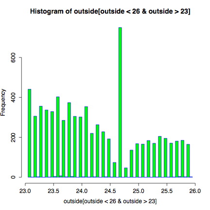
Still, what about the mystery that started our exploration? What is there such a spike around 24 degrees in outdoor temperatures? Maybe we should look at the histogram with some more care. In particular, we can use predicative criteria to index a vector, and narrow our histogram to just the temperature range of interest:
hist(outside[outside < 26 & outside > 23],
breaks=90, col="green" border="blue")
Looking at a close-up of the temperature spike, we see distinct troughs right next to the spike. It looks like if you would smooth the few tenths-of-a-degree region right around 24.7 degrees, you would almost get the expected occurences. Which brings us back, most likely, to odd rounding behavior within the thermometer instrument. Well, probably--we are still not sure. And even with some smoothing, there would still be a slight spike.
One of R's strengths is its ability to calculate linear, as well as
nonlinear regression models. To see a simple example, let us create
two vectors. x will be sample times in days measured from the
beginning of the data set, and y will be the corresponding outside
temperatures.
> y <- glarp$outside
> x <- 1:length(y)/(24*60/3)
We can fit a line to this data with
> l1 = lm(y ~ x)
> summary(l1)
Call:
lm(formula = y ~ x)

Residuals:
     Min       1Q   Median       3Q      Max
-29.4402  -7.4330   0.2871   7.4971  23.1355

Coefficients:
        Estimate Std. Error t value Pr(>|t|)
(Intercept) 10.2511014  0.0447748  228.95   <2e-16 ***
x           -0.0037324  0.0002172  -17.19   <2e-16 ***
---
Signif. codes:  0 `***' 0.001 `**' 0.01 `*' 0.05 `.' 0.1 ` ' 1

Residual standard error: 9.236 on 169489 degrees of freedom
Multiple R-Squared: 0.00174,    Adjusted R-squared: 0.001734
F-statistic: 295.4 on 1 and 169489 DF,  p-value: < 2.2e-16
The "~" syntax denotes a formula object. This in effect asks R to find
the coefficients A and B which minimize sum((y[i]-(A*x[i]+B))^2).
The best fit is when A is -0.0037324 (very close to flat slope), and B
is 10.2511014. Note, the residual standard error is 9.236, which is
about the same size as the standard deviation in y to begin with. This
tells us that a simple linear function of time is an extremely bad
model for outside temperature.
A better model might be to use sine and cosine functions with a periods of 1 day and 1 year. This we can do by changing the formula to
> l2 = lm(y ~ +I(sin(2*pi*x/365)) +I(cos(2*pi*x/365))
+             +I(sin(2*pi*x)) +I(cos(2*pi*x)) )
This formula syntax is a little tricky: Inside the I() calls the
arithmetic symbols have their usual meanings, so the first I(), for
example, is means: 2 times pi times x, divided by 365. The "+" signs
in front of the I() calls indicate not addition, but that the factor
following the + should be included in the model. The result can, as
usual, be displayed with the summary() command
> summary(l2)
Call:
lm(formula = y ~ +I(sin(2 * pi * x/365)) +I(cos(2 * pi * x/365))
                 +I(sin(2 * pi * x)) +I(cos(2 * pi * x)))

Residuals:
     Min       1Q   Median       3Q      Max
-21.7522  -3.4440   0.1651   3.7004  17.0517

Coefficients:
               Estimate Std. Error t value Pr(>|t|)
(Intercept)             9.76817    0.01306  747.66   <2e-16 ***
I(sin(2 * pi * x/365)) -1.17171    0.01827  -64.13   <2e-16 ***
I(cos(2 * pi * x/365)) 10.04347    0.01869  537.46   <2e-16 ***
I(sin(2 * pi * x))     -0.58321    0.01846  -31.59   <2e-16 ***
I(cos(2 * pi * x))      3.64653    0.01848  197.30   <2e-16 ***
---
Signif. codes:  0 `***' 0.001 `**' 0.01 `*' 0.05 `.' 0.1 ` ' 1

Residual standard error: 5.377 on 169486 degrees of freedom
Multiple R-Squared: 0.6617,     Adjusted R-squared: 0.6617
F-statistic: 8.286e+04 on 4 and 169486 DF,  p-value: < 2.2e-16
The residual error is still large (5.377), but we console ourselves in the fact that Colorado weather is notoriously unpredictable.
R provides still more tools for time series analysis. For example, we can plot the autocorrelation function for the living room temperature
> acf(ts(glarp$livingroom, frequency=(24*60/3)),
+     na.action=na.pass, lag.max=9*(24*60/3))
The embeded ts() function creates a time series object out of the
vector glarp$livingroom. The sampling frequency is specified in
samples per day. Not surprisingly the temperature is strongly
correlated when the shift is an integer number of days. Note also the
slightly larger peak at 7 days. This is caused by the fact that Brad's
thermostat sets the temperature differently on weekends, resulting in
slightly larger correlation with a 7 day window.
The home page for the "R Project for Statistical Computing" is:
http://www.r-project.org/
Several readers of my Charming Python column, being Python users, have expressed a particular fondness for the Python binding to R. Actually, there are two of them; RPy lives at:
http://rpy.sourceforge.net/
The older RSPython is also good, but my impression is that the RPy binding is better. RSPython can be found at:
http://www.omegahat.org/RSPython/
Either one of these bindings let you call the full range of R functions transparently from Python code, using Python objects as arguments to the functions.
The R web site contains extensive documentation, everything from tutorials to complete API descriptions. Two tutorials stand out of particular interest to those readers first encountering R:
"An Introduction to R": http://cran.r-project.org/doc/manuals/R-intro.pdf
And:
"R Data Import/Export": http://cran.r-project.org/doc/manuals/R-data.pdf
For what it is worth, on most systems you can launch a browser with
generated HTML pages for R documentation by entering help.start() at
the R command line.
A summary of the history of S annd S-Plus can be found at:
http://cm.bell-labs.com/cm/ms/departments/sia/S/history.html
Something about other stats packages: SPSS, SAS, Matlab, etc.
Coauthor David wrote a Charming Python installment on Numerical Python, which has a similar feel, and many of the same capabilities of R (R is considerably more extensive though):
http://www-106.ibm.com/developerworks/linux/library/l-cpnum.html
The temperature data and the Python script for converting the initial log format to a nicer tabular format can be found at:
http://gnosis.cx/download/R/basement.gz
http://gnosis.cx/download/R/lab.gz
http://gnosis.cx/download/R/livingroom.gz
http://gnosis.cx/download/R/outside.gz
http://gnosis.cx/download/R/unify-measures.py
To David Mertz, all the world is a stage; and his career is devoted to
providing marginal staging instructions. David may be reached at
[email protected]; his life pored over athttp://gnosis.cx/publish/.
Suggestions and recommendations on this, past, or future, columns are
welcomed. Check out David's book Text Processing in Python at
http//gnosis.cx/TPiP/.
Brad Huntting is a Mathematician completing a Ph.D. at the University of Colorado. You can reach him at [email protected].